Quick Start
Here we show two examples to illustrate how CoLFI works, and the readers can archieve their project quickly by modifing the examples. The code used to generate these examples can be downloaded here.
Using one dataset
The main process of using CoLFI includes preparing observational data and theoretical model, training the network, estimating parameters using the saved ANN chains or the well-trained network.
Let’s consider a general case, the simple linear model:
where a and b are two free parameters to be estimated, and y is the measurement. We first build a class object for this model:
class SimLinear(object):
    def __init__(self, x):
        self.x = x

    def model(self, x, a, b):
        return a + b * x

    def sim_y(self, params):
        a, b = params
        return self.model(self.x, a, b)

    def simulate(self, sim_params):
        return self.x, self.sim_y(sim_params)
Note
The class object must contain a simulate method, which is used to simulate samples in the training process.
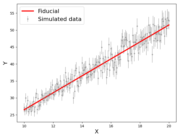
Then a data sample can be simulated as observational data, by using the function below:
import colfi.nde as nde
import numpy as np
import matplotlib.pyplot as plt

def get_data(x, a_fid, b_fid, random=True):
    np.random.seed(5)
    y_th = SimLinear(x).sim_y([a_fid, b_fid])
    err_y = y_th * 0.05
    if random:
        y = y_th + np.random.randn(len(x))*err_y
    else:
        y = y_th
    sim_data = np.c_[x, y, err_y]
    return sim_data, y_th

randn_num = np.random.randn()

a_fid, b_fid = 1.5, 2.5
x = np.linspace(10, 20, 201)
sim_data, y_th = get_data(x, a_fid, b_fid)

plt.figure(figsize=(8, 6))
plt.errorbar(x, sim_data[:,1], yerr=sim_data[:,2], fmt='.', color='gray', alpha=0.5, label='Simulated data')
plt.plot(x, y_th, 'r-', label='Fiducial', lw=3)
plt.xlabel('X', fontsize=16)
plt.ylabel('Y', fontsize=16)
plt.legend(fontsize=16)
After that, we can build a model instance and make some settings for parameter initialization:
model = SimLinear(x)
params_dict = {'a' : [r'$a$', np.nan, np.nan],
               'b' : [r'$b$', 0, 10]}
param_names = [key for key in params_dict.keys()]
init_params = np.array([[0, 5], [1, 3]])
where params_dict is a dictionary that contains information of the parameters, which include the labels and physical limits, and init_params is the initial settings of the parameter space.
Note
If the physical limits of parameters (the minimum and maximum values) is unknown or there is no physical limits, it should be set to
np.nan.
Finally, we can build a predictor and pass the data and model instance to it to train the network:
# nde_type = 'ANN'
# nde_type = 'MDN'
nde_type = 'MNN'
# nde_type = ['ANN', 'MNN']

chain_n = 3
num_train = 500
epoch = 2000
num_vali = 100
base_N = 500

predictor = nde.NDEs(sim_data, model, param_names, params_dict=params_dict, cov_matrix=None,
                     init_chain=None, init_params=init_params, nde_type=nde_type,
                     num_train=num_train, num_vali=num_vali, local_samples=None, chain_n=chain_n)
predictor.base_N = base_N
predictor.epoch = epoch
predictor.fiducial_params = [a_fid, b_fid]
# predictor.file_identity = 'linear'
predictor.randn_num = randn_num
predictor.fast_training = True

predictor.train(path='test_linear')
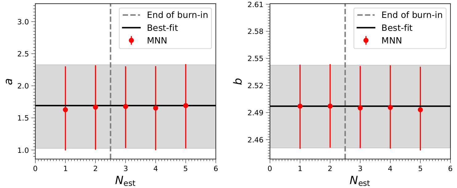
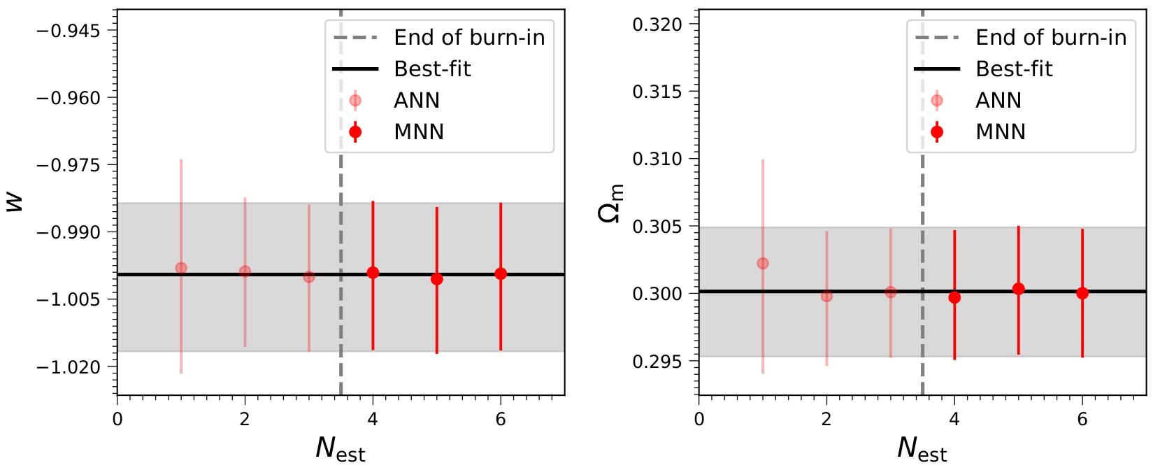
In the training process, the results which include the NDE model, the predicted ANN chain, and some hyperparameters and settings of NDE will be saved to the indicated folder. After the training process, we can plot and save the predicted parameters in each step by using the following commands:
predictor.get_steps()
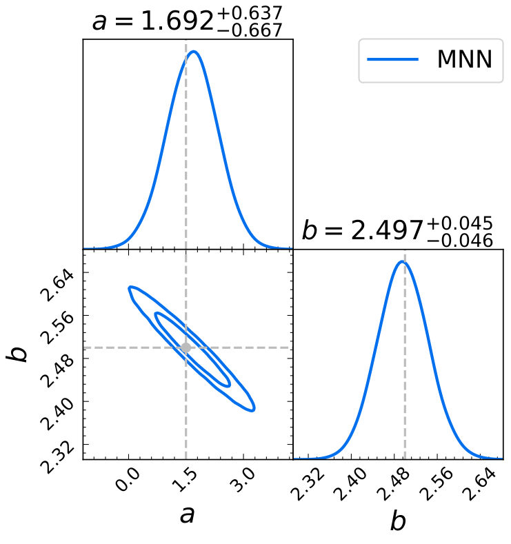
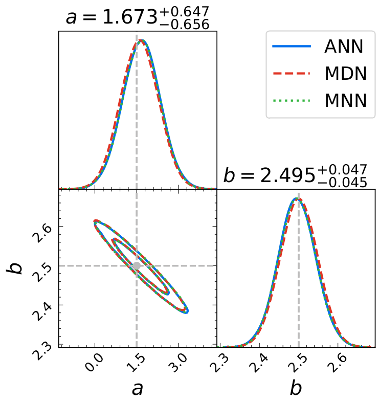
and can also plot the contours of the estimated parameters:
predictor.get_contour()
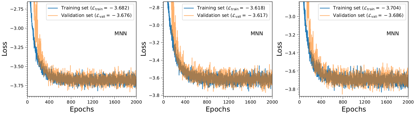
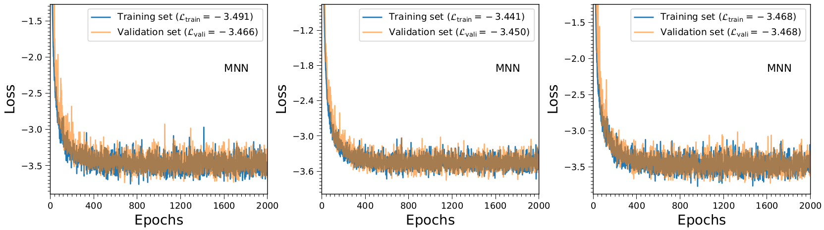
Besides, we can also plot the losses of the training set and validation set:
predictor.get_losses()
plt.show()
Note
The parameters are estimated using the ANN chains after the burn-in phase, and the chain_n is the number of chains to be obtained.
Also, the number of the training set (num_train) and the epoch should be set large enough to ensure the network
learns a reliable mapping. See the colfi.nde.NDEs module in Parameter estimation for details.
fast_training=True works well for simple models, but we recommend setting it to False for complex models.
In the training process, the results of each step will be saved, so it is possible to estimate parameters before the end of the training process. A file named predict_*.py will be saved automatically after the first step. Therefore, one can also execute the manuscript to see the estimation of parameters:
python predict_*.py
There are three NDEs (ANN, MDN, and MNN) in CoLFI, so we can also use ANN or MDN to estimate parameters. Besides, we can also use any two of them to estimate parameters, such as using ANN and MNN by setting nde_type = ['ANN', 'MNN']. In this case, the ANN will be used in the burn-in phase, and MNN will be used after the burn-in phase. After training ANN and MDN, we can plot all the results together by using:
randn_nums = [1.95713, 1.55973, 1.574] #the random number identifies each NDE

predictor = nde.PredictNDEs(path='test_linear', randn_nums=randn_nums)
predictor.fiducial_params = [1.5, 2.5]
predictor.from_chain()
predictor.get_contours()
plt.show()
Using multiple datasets
In practical scientific research, we may need to use multiple data sets to constrain the parameters, which is also possible for CoLFI. To illustrate this, we constrain parameters of \(w\)CDM cosmological model using the observations of Type Ia supernovae (SNe Ia) and baryon acoustic oscillations (BAO). We first build a class object for this model:
import colfi.nde as nde
import numpy as np
from scipy import integrate
import matplotlib.pyplot as plt

class Simulate_SNe_BAO(object):
    def __init__(self, z_SNe, z_BAO):
        self.z_SNe = z_SNe
        self.z_BAO = z_BAO
        self.c = 2.99792458e5

    def fwCDM_E(self, x, w, omm):
        return 1./np.sqrt( omm*(1+x)**3 + (1-omm)*(1+x)**(3*(1+w)) )

    def fwCDM_dl(self, z, w, omm, H0=70):
        def dl_i(z_i, w, omm, H0):
            dll = integrate.quad(self.fwCDM_E, 0, z_i, args=(w, omm))[0]
            dl_i = (1+z_i)*self.c *dll/H0
            return dl_i
        dl = np.vectorize(dl_i)(z, w, omm, H0)
        return dl

    def fwCDM_mu(self, params):
        w, omm = params
        dl = self.fwCDM_dl(self.z_SNe, w, omm)
        mu = 5*np.log10(dl) + 25
        return mu

    def fwCDM_Hz(self, params):
        w, omm = params
        H0 = 70
        hz = H0 * np.sqrt(omm*(1+self.z_BAO)**3 + (1-omm)*(1+self.z_BAO)**(3*(1+w)) )
        return hz

    def fwCDM_DA(self, params):
        w, omm = params
        dl = self.fwCDM_dl(self.z_BAO, w, omm)
        da = dl/(1+self.z_BAO)**2
        return da

    def simulate(self, sim_params):
        zz = [self.z_SNe, self.z_BAO, self.z_BAO]
        yy = [self.fwCDM_mu(sim_params), self.fwCDM_Hz(sim_params), self.fwCDM_DA(sim_params)]
        return zz, yy
Note that the measurement of SNe Ia is the distance modulus \(\mu(z)\) (fwCDM_mu), and the measurements of BAO are the Hubble parameter \(H(z)\) (fwCDM_Hz) and the angular diameter distance \(D_A(z)\) (fwCDM_DA). So, the outputs of the simulate method are \(\mu(z)\), \(H(z)\), and \(D_A(z)\). The parameters to be constrained are \(w\) (w) and \(\Omega_{\rm m}\) (omm). Then we generate mock observational using the method below:
def sim_SNe(fid_params = [-1, 0.3]):
    z = np.arange(0.1+0.05, 1.7+0.05, 0.1)
    N_per_bin = np.array([69,208,402,223,327,136,136,136,136,136,136,136,136,136,136,136])
    err_stat = np.sqrt( 0.08**2+0.09**2+(0.07*z)**2 )/np.sqrt(N_per_bin)
    err_sys = 0.01*(1+z)/1.8
    err_tot = np.sqrt( err_stat**2+err_sys**2 )
    sim_mu = Simulate_SNe_BAO(z, None).fwCDM_mu(fid_params)
    sne = np.c_[z, sim_mu, err_tot]
    return sne

def sim_BAO(fid_params = [-1, 0.3]):
    z = np.array([0.2264208 , 0.32872246, 0.42808132, 0.53026194, 0.62958298,
                  0.72888132, 0.82817967, 0.93030733, 1.02958298, 1.12885863,
                  1.22811158, 1.33017872, 1.42938629, 1.53137778, 1.63045674,
                  1.72942222, 1.80803026])
    errOverHz = np.array([0.01824, 0.01216, 0.00992, 0.00816, 0.00704, 0.00656, 0.0064 ,
                          0.00624, 0.00656, 0.00704, 0.008  , 0.00944, 0.01168, 0.0152 ,
                          0.02096, 0.02992, 0.05248])
    errOverDA = np.array([0.0112 , 0.00752, 0.00608, 0.00496, 0.00432, 0.00416, 0.004  ,
                          0.004  , 0.00432, 0.00464, 0.00544, 0.00672, 0.00848, 0.01136,
                          0.01584, 0.02272, 0.04016])

    sim_Hz = Simulate_SNe_BAO(None, z).fwCDM_Hz(fid_params)
    sim_Hz_err = sim_Hz * errOverHz
    sim_DA = Simulate_SNe_BAO(None, z).fwCDM_DA(fid_params)
    sim_DA_err = sim_DA * errOverDA
    sim_Hz_all = np.c_[z, sim_Hz, sim_Hz_err]
    sim_DA_all = np.c_[z, sim_DA, sim_DA_err]
    return sim_Hz_all, sim_DA_all

fid_params = [-1, 0.3]
sim_mu = sim_SNe(fid_params=fid_params)
sim_Hz, sim_DA = sim_BAO(fid_params=fid_params)
z_SNe = sim_mu[:,0]
z_BAO = sim_Hz[:,0]
obs_data = [sim_mu, sim_Hz, sim_DA]
After that, we can build a model instance and make some settings for parameter initialization:
model = Simulate_SNe_BAO(z_SNe, z_BAO)
params_dict = {'w'      : [r'$w$', np.nan, np.nan],
              'omm'     : [r'$\Omega_m$', 0.0, 1.0]}
param_names = [key for key in params_dict.keys()]
init_params = np.array([[-2, 0], [0, 0.6]])
Finally, we can build a predictor and pass the data and model instance to it to train the NDEs:
nde_type = ['ANN', 'MNN']
# nde_type = 'ANN'
# nde_type = 'MDN'
# nde_type = 'MNN'
chain_n = 3
num_train = 500
epoch = 2000
num_vali = 100
base_N = 500
predictor = nde.NDEs(obs_data, model, param_names, params_dict=params_dict, cov_matrix=None,
init_chain=None, init_params=init_params, nde_type=nde_type,
num_train=num_train, num_vali=num_vali, local_samples=None, chain_n=chain_n)
predictor.base_N = base_N
predictor.epoch = epoch
predictor.fiducial_params = fid_params
# predictor.file_identity = 'SNe_BAO'
predictor.fast_training = True
predictor.train(path='test_SNeBAO')
predictor.get_steps()
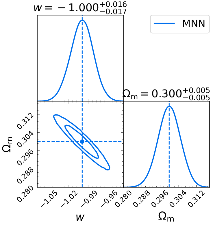
predictor.get_contour()
predictor.get_losses()
plt.show()
Note
The data used here have no covariance, so the covariance matrix (cov_matrix) is set to None. If the data have
covariance matrices, such as cov1, cov2, and cov3, they should be passed to the predictor by setting
cov_matrix=[cov1, cov2, cov3]. Furthermore, if some data sets have no covariance, such as the first data set, the
setting of the covariance matrix should be cov_matrix=[None, cov2, cov3].